Multiplier Effect
Multiplier Effect Overview
Money is the life-force of the economy. As money flows in the economy, it allows it to thrive and grow. This money flow is driven by spending. The interesting point is that money expands as it circulates in the economy. If a firm decides to inject $1 to the business, the impact to the economy is amplified by more than $1. This is known as the multiplier effect, and we shall explore what it is and how it works in this section. There are various multipliers – tax multiplier vs spending multiplier, balanced budget multiplier, and money multiplier. Let’s examine the marginal propensity to consume (MPC), and use it to explain the spending multiplier, taxation multiplier, and balanced-budget multiplier. The money multiplier will be discussed in another section.
Marginal Propensity to Consume (MPC) & Marginal Propensity to Save (MPS)
#1 Consumption and Saving Functions
The circular flow model shows how money flows from households to firms, and from firms back to households. Households (i.e. consumers) need to keep consuming goods and services to survive. This drive for survival forces households to use up their precious money to purchase the goods and services that they need from firms. In the process, money effectively flows from households to firms. This money is known as “Consumption” spending, and it is an important component of Aggregate Demand (AD).
Consumption spending is also important in driving the production of goods and services. Firms compete with each other to earn this money from households. In so doing, they need to make sure that the right goods, and in the right quantities, are produced. Firms, in the process of producing these goods, will cycle back some of this money to pay wages to households who worked in these firms. These wages will be an income source that fuels the next round of consumption spending.
Let us now dig in and build a more refined model on consumption, and use it to better understand what happens to money when it gets circulated in the economy.
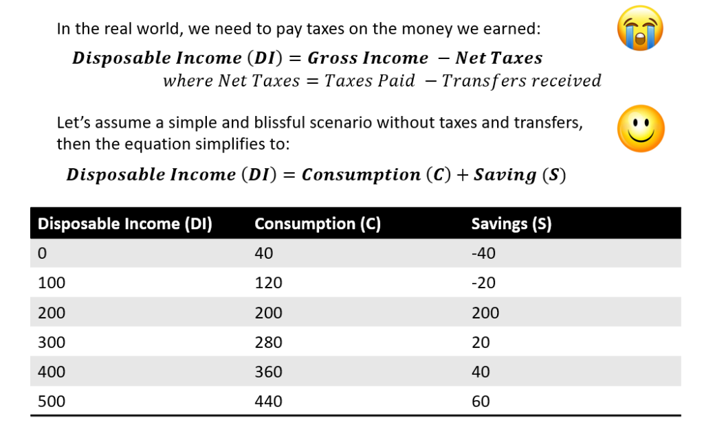
In a ideal world without taxes or transfers, disposable income (Yd) is equal to consumption and savings. This means that a household will use a portion of their income to purchase goods for consumption, and the save the remainder.
A typical household needs to consume some minimal amount of goods just to survive. Let’s assume that it’s $40. This is known as “Autonomous Consumption”. So, even without any disposable income, the household will borrow this amount and spend it to purchase the essential goods for consumption. Mathematically, the savings will be negative. This is also known as “dissaving”.
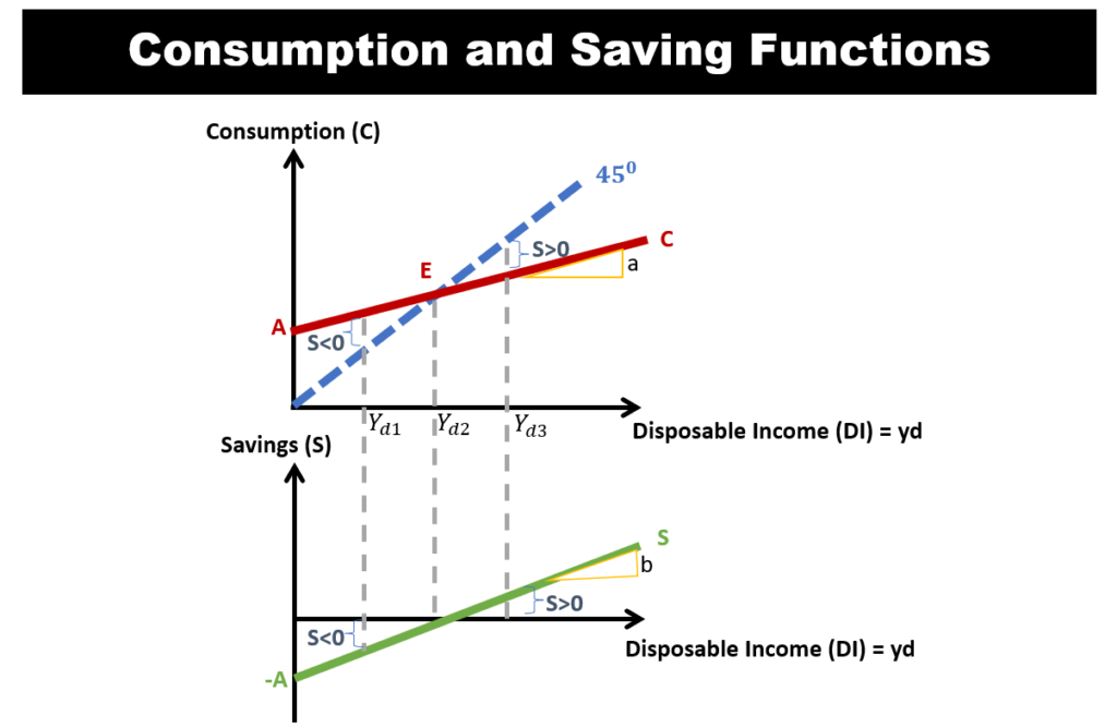
Let’s plot the consumption and savings in the table. This will yield the following consumption and savings functions on the right.
The consumption graph will be a linear function (C). The equation will be: C = A + a*Yd. Here, ‘A’ is the Y-intercept, and it also denotes the ‘Autonomous Consumption’ as mentioned above. ‘Yd’ denotes disposable income, and ‘a’ refers to the gradient.
Point E is where the household earns an income (Yd2) that exactly equals consumption. If the household earns more than Yd2, there will be saving. If they earn less than Yd2, there will be dissaving. We can similarly plot a savings function (S), and the equation will be: S = -A + b*Yd, where ‘b’ is the gradient of the savings function.
#2 Marginal Propensity to Consume (MPC) & Marginal Propensity to Save (MPS)
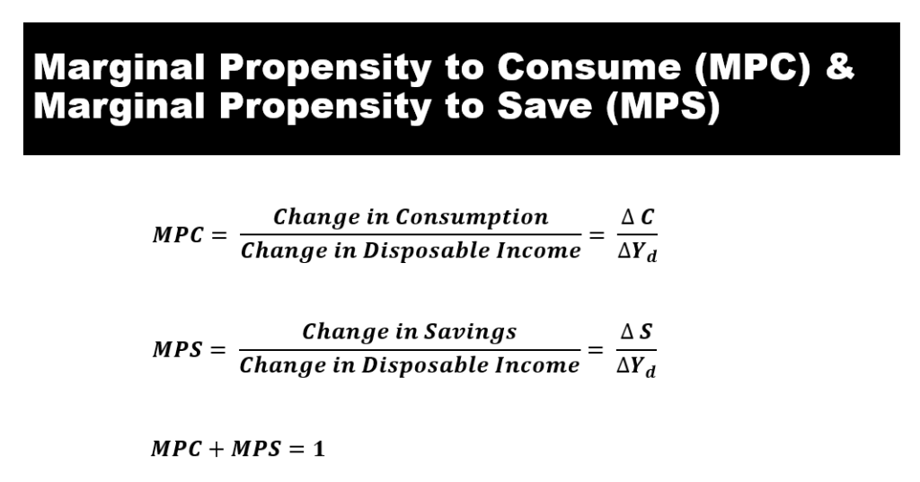
- Let’s focus on the gradients ‘a’ and ‘b’ from our charts above.
- We note that ‘a’ is the gradient of the consumption function. This is also known as the ‘Marginal Propensity to Consume (MPC)’. It denotes how much consumption changes given changes in disposable income.
- The gradient ‘b’ of the savings function is also known as the ‘Marginal Propensity to Save (MPS)’. MPS denotes how much do savings change given changes in disposable income.
- We should also note that MPC and MPS will sum to 1.
#3 Factors that affect Consumption and Saving
1. Weath
- When wealth increases, consumption function shifts upwards, while saving function shifts downward.
- This is because households can sell their some of their wealth assets to consume more goods even when their income remains constant.
2. Expectations
- When households are uncertain (i.e. ‘low expectation’) about future income, consumption shifts downward, while saving function shifts upward.
- This is because by saving more, then can even out their consumption in the uncertain future.
3. Household Debt
- Households can increase their consumption by borrowing (i.e. using debt).
- However, the more debt they used, the more disposable income they need to use to pay off debt. This will decrease consumption.
4. Taxes and Transfers
- If tax increases, both consumption and saving decreases.
- If government transfer increases, both consumption and saving increases.
The Multiplier Effect
Something interesting happens to money as it circulates in the economy. It actually expands!
#1 The Spending Multiplier
Let’s assume a simple case whereby there is only one household, and one firm in the economy. The firm sells goods to the household, and the household works for the firm. Let’s also assume that the household has an MPC of 0.8.
- Round 1: Let’s say a household receives an additional $100 wages increase from firms. Let’s assume the MPC is 0.8. This means that they will consume 80% of their income, and save the remainder. Hence, consumption spending is $80. This $80 becomes revenue to the firm who sold goods to the household.
- Round 2: That $80 that the firm earns become part of the wage that the firm needs to pay the household. The household will consume $64 (which is 80% of that $80 income, since their MPC is 0.8). This $64 then becomes revenue to firms who sold goods to the household.
- We note that after 2 rounds of circulation in the economy, the initial $100 money stock has already expanded to $100 + $80 + $64 = $244.
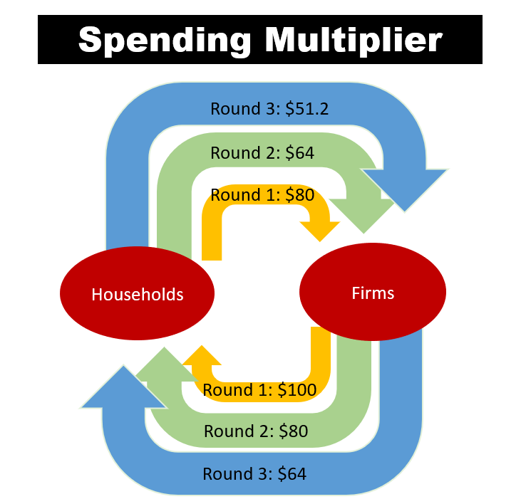
- The cycle repeats till all that initial $100 goes to 0. Mathematically, this is an arithmetic progression, and we can calculate the total money created using the formula: Spending Multiplier = 1/(1-MPC).
- Since our MPC is 0.8, So multiplier = 1/(1-0.8) = 5. This means that the initial $100 expands and becomes $500 as it circulates in the economy.
#2 The Taxation Multiplier
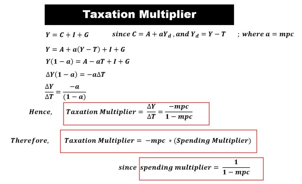
- When government raise taxes, there will be negative multiplier effect to the initial money stock. We call this the taxation multiplier.
- The taxation multiplier is smaller than the spending multiplier. The difference between these multipliers is actually the mps. One way to think about this is that the taxation is applied only after the first round of spending by consumers. So, there is a leakage in the form of savings as determined by the mps.
- The taxation multiplier is equal to -mpc/(1-mpc). The derivation is as shown in the diagram.
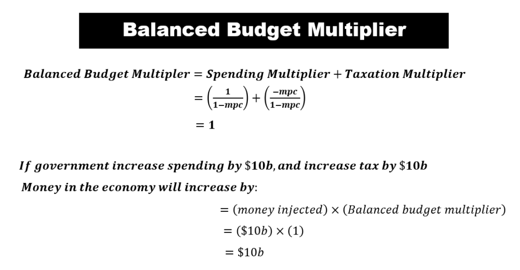
#3 The Balanced-Budget Multiplier
- A balanced budget means that the government spends exactly the same amount of tax collected.
- In a balanced-budget situation, will there still be money created?
- The answer is yes. The amount of money is created will be the amount of money injected. This is because the balanced-budget multiplier is 1. The derivation is as shown in the diagram.