Utility and Indifference Curve
Utility represents our satisfaction from consuming goods and services
The concept of utility is central to economics. It is used to model our needs and wants, and there is no known limit to that. We always need more – the more things we consume, the happier we are, and therefore the higher our ‘utility’. In order words, ‘utility’ is a measure of our ‘satisfaction’. However, this concept is planted in a framework of resources scarcity, that places an upper limit to how much we can enjoy our needs and wants. What’s the result? The result is that we have to make choices — we need to figure out the best way to maximise our satisfaction given the constraints of resources. Doing so make us “rational”. In other words, a “rational consumer” will attempt to achieve some equilibrium that can enable us to maximise our utility by consuming a basket of goods and services without busting our budget.
The law of diminishing marginal utility
Another thing that we need to know about ‘utility’ is that there is not linear. The more we have, the more we enjoy, but at a lesser rate than before. Formerly, this is known as the ‘Law of diminishing marginal utility’. It states that the additional units of satisfaction derives from every additional units of the good consumed will diminish as we consume more and more of the good in one setting. That is, as consumption increases, marginal utility will fall.
Introducing the indifference curve
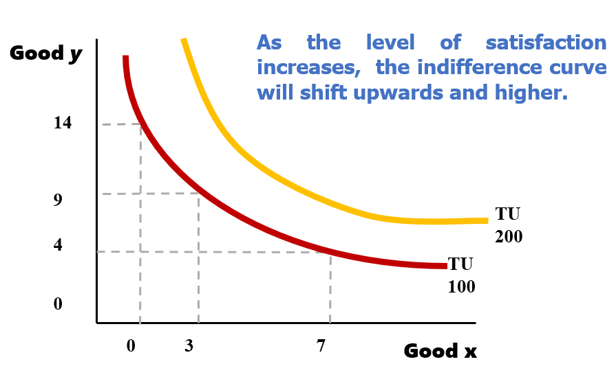
We can combine the concepts of utility and law of diminishing marginal utility together into a useful model, called the ‘indifference curve’. An indifference curve shows the various possible quantity combinations of two goods (x and y) that will give the consumer (that’s us) the same level of satisfaction. In other words, any points along on the indifference give us the same level of utility. A graph can have an infinite number of indifference curves, but these indifference curves cannot intersect with one another.
The indifference curve is negatively sloped, i.e. it slopes downwards from the left to right. This is because of the concept of opportunity cost. Opportunity cost can be defined as the next best alternative forgone. When demand for the good x increases, the consumer has to give up good y.
Note also that the substitution of x and y is not linear, and this encompass the idea of diminishing marginal utility. For instance, at high abundance of Y, we may be willing to give up a lot of Y just to gain a small amount of X.
As the level of satisfaction increases, the indifference curve will shift upwards and higher. That is, the higher the indifference curve, the higher the level of our satisfaction.
Introducing the budget line
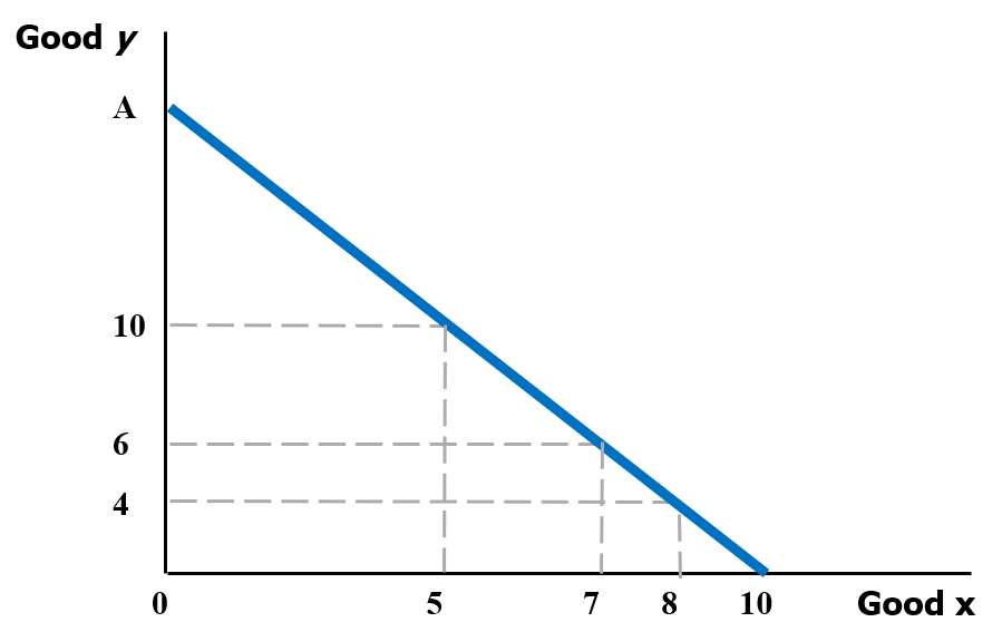
The budget line can be defined as a line that shows the combinations of any two goods that can be bought, given the level of income and the prices of both goods.
If we used up all our monetary resources to purchase goods X and Y, then we will fall along this budget line.
Any points below the budget line means we have purchase some combination of X and Y, but we still have some savings left.
Any points above the budget line refers to combinations of goods beyond what we can afford.
Everything together now...
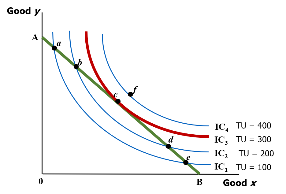
Consumer equilibrium is achieved when the indifference curve is tangent to the budget line. At this point, combination c is best possible point or the optimum combination based on the budget available. It lies on an indifference curve IC3, the highest indifference curve that we can achieve based on our budget constraint.
Note that points a, b, d, and e would not allow us to maximise our utility as the utility function, as indicated by the indifference curves, is much lower than that of IC3. This would not make us a ‘rational consumer’ would it?
Point f lies on an indifference curve that is higher than IC3, but it is beyond what our budget allows.