Unemployment-Inflation Tradeoff

Trade-off between Inflation and Unemployment

In previous sections, we learnt about inflation and unemployment. These were presented as independent siloed concepts. In reality, there is a trade-off between inflation and unemployment. in this section, we shall look at this trade-off in terms of the Phillips Curve. We shall also use the Phillips Curve to analyse stagflation.

Phillips Curve

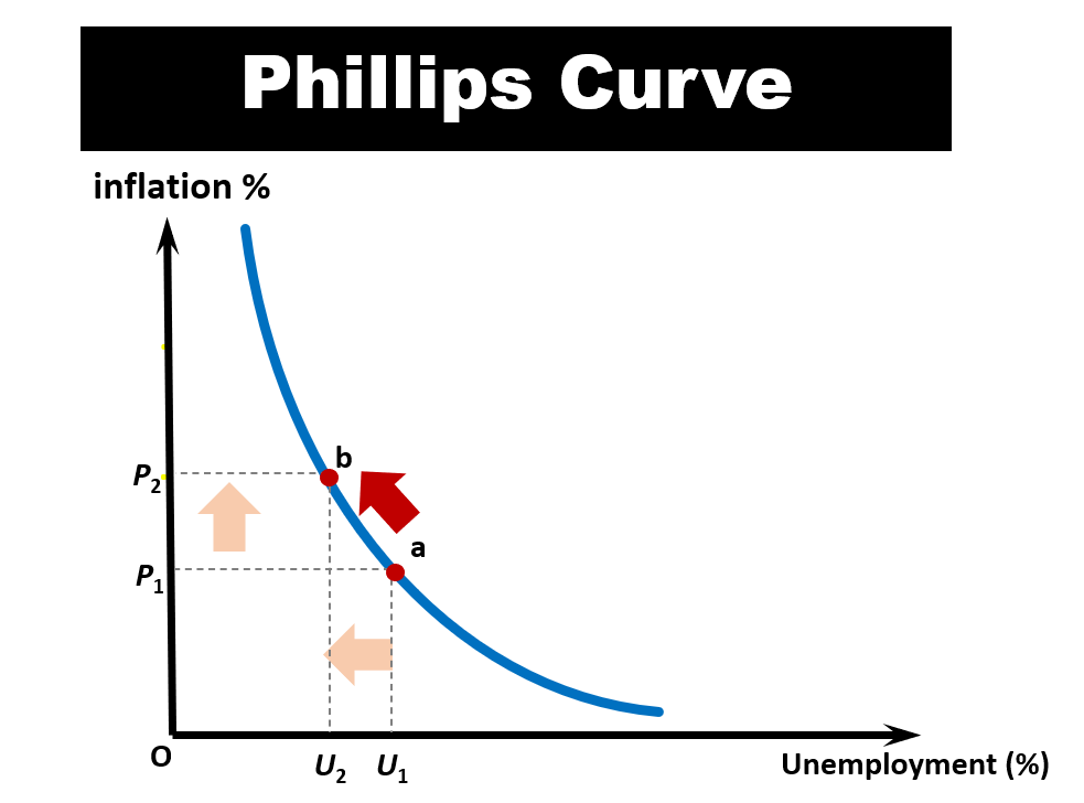
Williams Phillips was the first to note the negative relationship between inflation and unemployment in 1958. Phillips studied wage inflation and unemployment in the United Kingdom using data from 1861 to 1957. He argued that when unemployment rate is low, firms would raise wages to compete for scarce labour. Conversely, when unemployment rate is high, firms need only to offer low wages to hire the labour they need. This inverse relationship between inflation and unemployment is known as the Phillips Curve. Although the Phillips Curve was originally focused on wage inflation, it was later extended by other economists to analyse inflation in general.

Empirical Evidence and Supporters of the Phillips Curve

Following Phillips’ 1958 seminal paper, there were a lot of empirical studies supporting the inverse relationship between general inflation and unemployment. Many famous economists, including Paul Samuelson and Robert Solow believed that this relationship was stable and permanent, and hence promoted it. Fundamentally, there is a strong theoretical foundation supporting the Phillips curve from the Keynesian view point. While governments may not be able to control both unemployment and inflation at the same time, but they can be reined in them within reasonable levels. For instance, if government has the objective of lowering unemployment to a certain target, they can use fiscal and monetary policies to increase aggregate demand, while accepting slightly higher inflation as a trade-off.

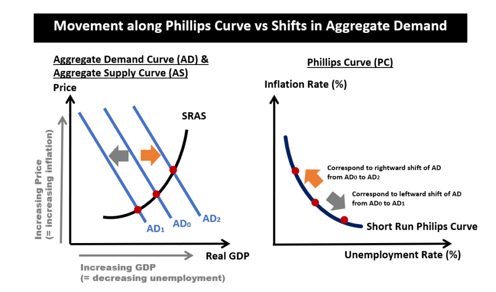
Let us know relate the movement along the Phillips Curve with shifts of the Aggregate Demand curve. First of all, let’s call the Phillips Curve the ‘Short-run Phillips Curve’ (we shall see why later).

An increase in aggregate demand (from AD0 to AD2) will increase GDP. This means that economy is thriving, and that a lot of consumers are spending in the economy. Hence, firms will need to hire more labour to produce more goods and services to keep up with the demand. In addition, firms may even need to pay higher wages to attract the labour they need, thereby contributing to inflation. In this scenario, the people in the labour force will have less problem finding jobs, and hence unemployment rate will decrease. In summary, a rightward shift of the AD curve corresponds to a leftward movement along the Short-run Phillips Curve.
An decrease in aggregate demand (from AD0 to AD1) will lead to a decrease in the GDP of the economy. This means that consumers have less money to buy goods and services. Firms would also cut back on production and costs (including wages) and even lay off excess staff, leading to higher unemployment. In summary, a leftward shift of the AD curve corresponds to a rightward movement along the Short-run Phillips Curve.

Monetarist View on The Phillips Curve

While there were many patrons for the Phillips Curve model, it also had its fair share of detractors. Cases in point include monetarists such as Edmund Phelps and Milton Friedman. They argued that in the long run, rational employers and rational workers will pay attention to only real wages, and will adjust their employment decision accordingly. Note that real wages means that nominal wages have been “inflation-adjusted”. In other words, there is no inverse relationship between inflation and unemployment in the long run where everyone is “rational”. The Phillips Curve that denotes the inflation-unemployment trade-off is simply a short-run phenomenon. In the Long Run, both the Phillips Curve and the Aggregate Supply would be vertical.

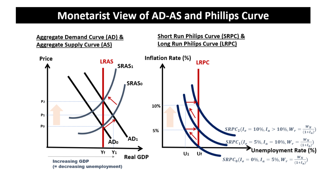
Let’s unpack the monetarist argument on the Phillips Curve. Suppose the economy is initially at full employment level Uf, with prices at P0, and inflation at 0%. This corresponds to SRPC0 in the Phillips Curve and AD0 and SRAS0 in the AD-AS model. If the government wants to reduce unemployment to U1, they can use expansionary fiscal policy (or monetary policy) to increasing Aggregate Demand. For simplicity, let’s assume that the government implements the expansionary fiscal policy by dishing out a road construction project to private sector . Here’s the step-by-step run down of what may happen:

Step 1: Firms need labour to complete the project and are willing to pay higher wages to entice workers. This increases overall prices from P0 to P1, and inflation increases from 0% to 5%. Some workers accept the job due to higher nominal wages (WN). Hence unemployment rate reduces from Uf to U1. This corresponds to an increase in output from Yf to Y1 due to an increase in AD from AD0 to AD1.
Step 2: Later, these workers realise that goods are now more expensive. That means that their expected inflation (Ie) of 0% is incorrect. They known now that actual inflation (Ia) is at 5%, and that their real wages are in fact lower than their nominal wages (i.e. real wages = nominal wages / (1.05)). These workers are not prepared to work at this lower real wage and decides to withdraw from their job and become unemployed again. This withdrawal of labour will increase the unemployment rate from U1 back to Uf. This corresponds to a rightward shift of the Short-Run Phillips curve from SRPC0 to SRPC1, and a contraction of the Short-Run Aggregate Supply curve.
We can note that the result is increased inflation, while the unemployment rate remains unchanged ay Uf, and output remain unchanged at Yf. The cycle will continue further if the government again attempt to use expansionary policy to lower the unemployment rate below Uf. Regardless how many times the cycle repeats, it will simply result in higher and higher inflation.
Monetarists from the adaptive expectation school argue that there can be short-term trade-off between inflation and unemployment.
Monetarists from the rational expectation school argue that there is no trade-off even in the short term, as rational workers have full knowledge of actual inflation rate and realise that real wages are actually the same. They will hence not be fooled into the job market.

Stagflation

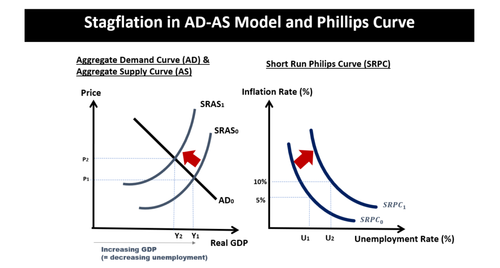
In the 1970s, something happened that shook the foundation of the Phillips Curve. There was a concurrent increase in both inflation and unemployment. This twin misery phenomenon is now known as “Stagflation”.

In terms of the Phillips Curve, stagflation is depicted as a movement in the northeast direction. This will lead to an increase in both unemployment and inflation at the same time.

In terms of the AD-AS model, stagflation is shown as contraction of the Short-run Aggregate Supply (SRAS) curve from SRAS0 to SRAS1.

#1 Causes of Stagflation

There are many explanations for the 1970s stagflation, and suspects include:

oil supply shock- created by oil embargo when OPEC monopolized prices.
wage-controls that artificially kept inflation low to limit domestic problems resulting from Vietnam war were lifted. That led to a significant escalation of business costs and prices of goods.
decline in productivity;

#2 Controlling Stagflation

Prioritizing inflation – since it is not possible to reduce both inflation and unemployment at the same time, the monetarists argued that we should choose to reduce inflation. The problem is that there may be higher unemployment in the short run.
Supply-side solutions — the idea is to increase long-run aggregate supply. There are several aspects of supply-side policies:

(a) investment in human capital (e.g. education, healthcare) to increase productivity;
(b) tax reduction – to incentivize motivation and risk-taking;
(c) investment in R&D to improve productivity;
(d) reduction in government regulations that stifle business growth and expansion.